The Math Behind RL for LLMs - Part 1, Foundations

Reinforcement Learning is an integral part of producing frontier LLMs, applied in multiple ways at different stages of post training. Given it drives so much of LLM behavior, it’s valuable for all of us to understand how it works.

The trouble is, RL is technical, it has a long history with many iterations, and it’s still rapidly evolving. As is the case with many technical fields, RL is built on multiple layers of concepts. Modern papers necessarily use the last layer of concepts. As someone new to the field, you might start by building a basic RL pipeline using Claude or Codex.

But you know that doesn’t build understanding, you need to engage with the equations yourself. So you follow the citation graph backwards, until you’re reading some terse paper written in the 90’s that is formatted so arcanely you have to screen shot it for your LLM. You’re sitting there asking yourself, what do I actually need to know? You’re exhausted by a big bag of algorithms and approaches, unsure which ones matter.

This post solves that problem, and teaches you RL so you understand it properly. We don’t skip out on any of the maths, and build a good base of RL fundamentals, but we also don’t get distracted by the complete history of RL. You are going to build the strong conceptual structure needed to go from states and actions, all the way to the various flavours of RLHF and RLVR.

States and Actions

There is a standard abstract model¹ used to represent Reinforcement Learning problems. Although RL in LLMs might look different, it is still based upon this abstract model. Given our goal of getting to LLMs, this section is deliberately brief, focusing on the essentials. If you want more, Lilian Weng’s blog post, or Sutton and Barto’s book are both excellent.

Reinforcement Learning is loosely inspired by real biological learning systems like animals. Birds can learn which types of flowers yield the most nectar, or the risk associated with certain types of predators. Dogs can learn all manner of tricks to please their owners, or learn that they should not go near wire fences because they give electric shocks.

In RL we model the environment (the world) as a set of states. The agent (the dog) can take various actions, which causes it to arrive at different states. Each state yields a reward (sometimes positive, sometimes negative, usually zero). The agent’s goal is to take actions to maximize the return (sum of future rewards).

To make this concrete, let’s consider a simple example of a dog (agent) on a farm (environment). The dog loves to be with its owner, but the dog is currently on the other side of the fence (the start state). From the start, the dog can take three actions:

1. run to the the fence state, receiving an electric shock (R = -4)

2. run to the end of the field state, which has rough terrain consuming energy (R = -1)

3. take a nap to stay in the start state (the circular arrow), no cost but no gain

Once the dog is either at the fence or gate state, being a small dog, they can pass through and reach the owner (the terminal state) This also happens to be the only place in the environment the dog receives a positive reward (R = -5).

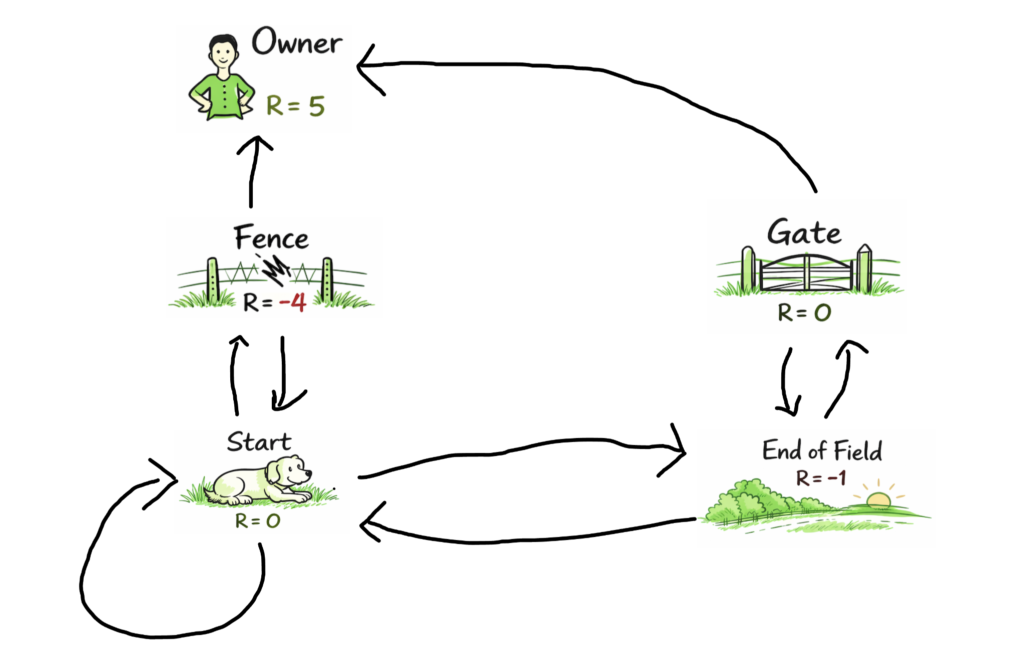
Our pretty little example is easy to understand, but we need to be more precise to get the right conceptual model. First of all, the diagram above represents our dog’s entire reality, not a specific situation it encounters. This dog’s entire day consists of starting one side of the fence, moving through a series of states, and ending with the owner.

Secondly, you might imagine the dog to see or smell the owner, or have spatial knowledge of the farm. While it is possible to imbue such prior knowledge into our dog agent, in the basic setup we assume no prior knowledge. This means the dog does not know the paths to the owner, it does not know the fence gives it a shock, in fact it does not even know that it likes its owner. The dog has to reach those states to receive rewards, and learn they are desirable.

So what can our dog, who knows absolutely nothing, achieve in one day? Not a lot. He’ll randomly move around the farm states observing rewards. Maybe getting shocked, maybe running to the end of the field, experiencing joy when it reaches the owner. The next day is exactly the same, the dog knows nothing, he explores, collects rewards. A better word for “day” is rollout.

After a batch of rollouts (days), we have collected enough reward observations for an update. Our dog agent has a model of reality, it will be updated slightly to favour the actions which maximize reward. Relatively speaking, the dog will be more likely to choose the more rewarding path. After enough batches and updates, the dog should (ideally) converge on the optimal strategy of running to the end of the field, through the gate.

Our dog is now fully trained, he can now exploit the optimal strategy he learned, always avoiding the fence and just running around. I designed this example to (very lightly) express the original conceptual model RL. When wrestling with the equations and code below, it will be useful to come back to, knowing that modern RL is downstream of it.

Glazebot

In this section we’ll get into the actual algorithms + equations and write some code. We’ll train a little chatbot called glazebot. Unlike most toy RL problems, this one is token generation flavoured. The intent is to introduce you to the details of a simple token problem you can hold in your head, so that you can tackle the more general case of LLMs confidently.

We’ll work through the equations, and then show the code bit by bit. Try to hand write the code yourself first², without looking at the code I supply. Trying to figure it out yourself, whether you get it right or not will give you a much deeper, sticky understanding. If you do this, you’ll have a solid basis for when things get more complex.

The code for glazebot can be found here, keep the model tracker module but delete the main script and try writing it yourself.

Glazebot operates in a small token space with hardcoded terminal states. Here is the world as seen by glazebot (as generated by Claude):

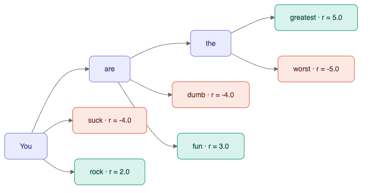
There are 6 possible sequences, correspond to the 6 terminal states:

• You rock (reward +2)

• You suck (reward -4)

• You are fun (reward +3)

• You are dumb (reward -4)

• You are the worst (reward -5)

• You are the best (reward +5)

There are only three non-terminal states:

• You

• You are

• You are the

Technically, the whole sequence is part of the state (not just the last token). For our simple problem, there is only one path to each token, so using the token to represent the state works. Remember that when we get to LLMs, we will need the whole sequence to represent the state. For now token == state.

There is no prompt and only one starting state “You”. This makes the optimal strategy very simple, always output “You are the best”. Nonetheless, our little agent does not know that, it needs to learn it.

State and Model

We can represent a token as follows:

@dataclass
class Token:
    word: str
    children: Optional[List[Token]] = None
    reward: Optional[float] = None

The word is the next token value itself, e.g. “You”. The children are all possible tokens that can come after that token. The reward only exists for terminal nodes. Starting with “You”, we have the entire tree our little agent needs to explore. We can now use this data structure to create a hardcoded state transition diagram of tokens, our tree that starts from “You”:

def create_token(
  word: str,
  children: Optional[List[Token]] = None,
  reward: Optional[float] = None) -> Token:
  # Terminal Tokens must have no children and a reward
  if children is None or reward is not None:
    assert children is None and reward is not None  
    return Token(word, reward=reward)
  # Non-terminal token
  return Token(word, children=children)

def create_tree() -> Token:
  """
  Create the state graph, returning the root level token "You".
  """
  greatest = create_token("greatest", reward=5.0)
  worst = create_token("worst", reward=-5.0)
  the = create_token("the", children=[greatest, worst])
  lame = create_token("dumb", reward=-4.0)
  fun = create_token("fun", reward=3.0)
  are = create_token("are", [the, lame, fun])
  suck = create_token("suck", reward=-4.0)
  rock = create_token("rock", reward=2.0)
  return create_token("You", [are, suck, rock])

That’s the RL problem we wish to optimize, but we need a model now. Given our small setup, we have the luxury of being able to have a parameter per action³. There are only 3 non-terminal states; “You” and “are” with 3 actions each, and “the” with two actions.

To explore action space with reinforcement learning, we’ll need those parameters to correspond to probabilities. For a given state (e.g. “You”) we would like that if one action’s parameter is higher, relative to the others, it should have a higher probability. For that purpose we use the softmax function:

Where $w_{0}$ is the parameter for the action which takes us to “rock”, $w_{1}$ for that which takes us to “suck” and $w_{2}$ for “are”. Notice that no matter the values for each $w_{j}$. This will always produce a valid probability distribution. Of course if $w_{0}$ is too much larger than $w_{1}$ and $w_{2}$ $p("rock" | "You") \approx 1$ and we’ll never sample anything else. We can introduce a temperature parameter to control for the smoothness of the probabilities:

That is all there is to our model, 3 different softmax functions at the 3 terminal states. Each ModelNode is represented by a single action weight array:

class ModelNode:

  def __init__(self, num_action):

We can then create both our state transition object, and our model from the main script:

  you = create_tree()
  # Create model manually for simplicity
  model = {"You": ModelNode(3), "are": ModelNode(3), "the": ModelNode(2)}

REINFORCE

If one could call a single algorithm the foundation of modern RL it would be the REINFORCE algorithm developed by Ronald J Williams in 1992. This is where policy gradients were first proposed. These policy gradients tell our action parameters how they need to update, to maximize our expected sum of rewards. Modern RLVR really isn’t that different to the REINFORCE algorithm.

Quick Aside - Notation and Indexing

This section gets math heavy. Equations are concise, great at distilling the essence of things, but notation is notoriously non-standardized. Let’s clarify a few things:

• All number quantities should be assumed to be scalars unless otherwise stated. For example the return G, or the output of the Value function $V_{\tau \sim p_{\theta}}(x_{t})$ are both scalars.

• There are 3 indices we use, batch index (which sample), sequence index (where in sequence) and action index (which next token). We always index in that order (batch first, sequence second, action last).

• As variable indices, we use i for the batch dimension t for the sequence dimension, and j for the action dimension. There are n elements in each batch, T elements in the sequence, and v possible actions⁴.

• Indices are only shown if they are needed. If there is no index, it means we could be referring to any value along that dimension. So while $G_{i, 2, j}$ means the ith rollout, at token position 2, for next token choice (action) indexed by j, we’ll just write G if we don’t care about the specific indices.

• When there are only 1 or 2 indices; the context, or the specific use of i, t, or j, will make it clear which dimensions are being indexed.

Maximizing Returns

In one rollout, we generate a trajectory (sequence) of tokens. We can write that as $\tau = x_{0}, x_{1}, ... x_{t}$ for a sequence of length T. All the softmax weights induce the probability distribution across all possible sequences. We write $\theta$ as a catch all for all our weights. When we say $\tau \sim p_{\theta}$ we are saying the sequence is a probability distribution that depends on our weights

We call the sum of rewards the return, which is denoted as $G_{0}$ (return at t=0). We want to maximize the expected return, which we also call the value:

Ultimately, $V_{\tau \sim p_{\theta}}("You")$ is the state we are about, because it is our starting state, but we also need to express the value of other states:

We can then the expected return at one state, recursively in terms of the others:

This is useful because it shows us we can increase $V_{\tau \sim p_{\theta}}("You")$, by increasing the probability of the more valuable downstream states. More generally, we can express $V_{\tau \sim p_{\theta}}$ recursively for any token $x_{t}$ with $v$ possible next tokens⁵:

The index j allows us to sum across all possible next tokens e.g. $x_{1,0} = "are"$. Notice we also introduced a discount factor $0 < \gamma \leq 1$ . For $\gamma < 1$, this induces a preference for more immediate rewards over later rewards (shorter token sequences). However in then training of LLMs it is often set to $\gamma = 1$

Finally, for the sake of optimization will need to express V for a particular parameterization, a particular value of $\theta$. In our glazebot case, $\theta$ just represents the list of weight vectors, where each individual vector $w$ is at a non-terminal state. We’ll change our notation to incorporate $\theta$:

Before we move to finding the gradients, those familiar with the foundational RL will note that states, actions, and the $Q$ functions are all missing. That general notation isn’t required for LLMs and frankly it is distracting. The LLM has a single root BOS token, and each state is an entire sequence, consequently the state transition diagram is just a tree, so $Q$ is not required⁶.

Deriving Gradients

It’s tempting to look at our equation for $V(\theta; x_{t})$ and simply differentiate w.r.t to $p(x_{t + 1, j}| x_{t})$, which itself is just the softmax over $w$, which is easy to differentiate. Vanishing gradients aside, this would totally work for glazebot, because we can compute $V(\theta; x_{t})$ exactly for all possible states.

However the state space for an LLM grows exponentially in the number of tokens, computing $V(\theta; x_{t})$ exactly would not work. To stay closer to the way we train LLMs, we instead sample rollouts and take the mean to estimate $V(\theta; x_{t})$. This is very easy to do:

This is an unbiased estimator of $V(\theta; x_{t})$, but it creates a new problem. By sampling from $p(x_{t + 1, j}| x_{t})$ we remove it from the expression. This is a problem because $p(x_{t + 1, j}| x_{t})$ was the only influence $w$ had on the value function. To resolve this we use the log gradient trick, which we’ll go through now, starting with the original expectation based expression:

We’ll focus on the derivative, with respect to a specific weight vector $w$ to keep things concrete. For glazebot, $w$corresponds to the non-terminal state $x_{t}$. We use a slightly unconventional symbol to represent differentiating by $w$, $\Delta_{w}$:

Looks great but can’t sample from this because there is no $p(x_{t + 1, j}| x_{t})$ term, however we know that:

rearranging we have:

Plugging back in:

This quantity includes, $p(x_{t + 1, j}| x_{t})$ so we can therefore sample particular actions. We can then compute a gradient empirically for the $w_{k}$at each non-terminal state:

The expression $\Delta_{w_{k}}\log\lbrack p(x_{t + 1, i}| x_{t})\rbrack$ is a simple v dimensional vector with a nice simple interpretation. At each index j of that vector we have:

$y_{j} = 1$ when action j was the action chosen, 0 otherwise. This gives us the gradient contribution of a single rollout and single state transition in that rollout, on a single weight parameter.

Suppose the return $G_{ t + 1}$ is positive, then:

1. For the selected action: $(1 - p(x_{t + 1}| x_{t}))G_{ t + 1}$ push its weight up , particularly if its probability is low.

2. For the non-selected action: $- {p(x_{t + 1}| x_{t})G}_{ t + 1}$push their weights down, particularly if their probabilities were high.

Note if $G_{ t + 1}$ is negative (e.g. the return from taking action “suck at “You”) the effect is the opposite. The weight scalar for the “suck” action at state “You” will go down.

Advantage Optimization

Before we move to implementation, we are missing one improvement. First, suppose the non-terminal nodes “You are the” and “You are” had optimal weights⁷. When this is true, all of the three choices from “You” have positive expected returns (values):

• You rock (reward +2)

• You are fun (reward +3)

• You are the best (reward +5)

This still works, it would be better to optimize for the action that has a better return on a relative basis, i.e. that with a higher advantage. To do this, we simply subtract the expected value of the next state, from the return:

which as shown previously, is just estimated with the mean at the next state: $V(\theta; x_{t + 1}) = \frac{\gamma}{n}\sum_{i = 1}^{n}G_{t + {1, i}}$

So our chosen action update for an individual point becomes:

$(1 - p(x_{t + 1}| x_{t}))(G_{ t + 1}$- $V(\theta; x_{t + 1})$)

Now, at state $x_{0} = "You"$ the only choice that produces a positive update is “are”. Overall, using the advantage estimate instead of the raw return reduces variance, speeding up convergence to the optimal solution.

Summarizing

• For glazebot, as shorthand we represent states by their token $x_{t}$ (e.g $x_{1} = "rock"$)

• The expected return of each state is given by the value function $V(\theta; x_{t})$, which we simply estimate with its sample mean: $V(\theta; x_{t}) = \frac{\gamma}{n}\sum_{i = 1}^{n}G_{t + {1, i}}$ over a batch of n rollouts.

• The value function is a recursive function of the expected value of later tokens

• We use the log gradient trick to get a gradient w.r.t to the weights that can be samples, that gradient is $\Delta_{w_{k}}V(\theta; x_{t}) = \frac{\gamma}{n}\sum_{i = 1}^{n}\Delta_{w_{k}} \log\lbrack p(x_{i, t + 1 }| x_{t})\rbrack G_{i, t + 1}$

• However, we can reduce variance maximizing the advantage instead of the value:
  $\Delta_{w_{k}}V(\theta; x_{t}) = \frac{\gamma}{n}\sum_{i = 1}^{n}\Delta_{w_{k}} \log\lbrack p(x_{i, t + 1 }| x_{t})\rbrack(G_{i, t + 1} - V(\theta; x_{t + 1}))$

• We can now use gradient ascent to train our weights.

There were a lot of details to get here, but ultimately the update is very simple. As we explore all the different flavours of modern RL, you’ll see they basically boil down to this. Estimate the expected advantage, push the weight up if the return from the action is positive, down if it’s negative, exponentially reducing that update as $p$ approaches 1 or 0.

Implementation

The implementation is left as an exercise to the reader. As previously mentioned, the code is here. Please delete the contents of the main script and implement it yourself.

To give you some structure, we’ll define the HyperParmeters object and the subs for the key functions you should implement. There is also a weight tracker that allows you to see how your run converged (this was AI generated, don’t write it yourself!).

For the hyperparameters, the only parameter we haven’t mentioned so far is the learning rate lr, which specifies the strength of the update:
\

@dataclass
class HyperParameters:
  epochs: int = 90
  batch_size: int = 10
  lr: float = 0.5
  temperature: float = 3.0
  gamma: float = 1.0
  use_advantage: bool = True

The batch size is actually a bit more nuanced. In the equations above we pretended each state has the same batch size. In reality only “You” has the full batch size of n rollouts. Each of the other states is not always visited, so their batch sizes is actually lower⁸. This issue is caused by the fact our parameters are state specific, which is not the case.

Here is the high level main function, which you are welcome to either copy or try to implement yourself. Your key implementation challenge is to write the rollout and update functions and get Glazebot working. You should see the weights converging on a solution that mostly outputs “You are the best”. After that, you’ll be in a strong position to move onto LLMs.

def main():
  np.random.seed(58641)
  you = create_tree()
  # Create model manually for simplicity
  model = {"You": ModelNode(3), "are": ModelNode(3), "the": ModelNode(2)}

  # Training
  hp = HyperParameters()
  tracker = ModelTracker(hp.temperature)
  tracker.record(0, model)  # Record initial weights
  for e in range(1, hp.epochs + 1):
    # 1) Rollout
    average_return = rollout(hp, model, you)
    # 2) Update
    update(hp, model)
    # 3) Monitor
    tracker.record(e, model)
    print(f"EPOCH: {e}, AVERAGE RETURN: {average_return}")
    print("")

  tracker.plot()

LLM Foundations

Let’s consider what would happen if we tried to apply the Glazebot approach to a frontier AI model. The walls we run into will be amusing, and motivation for the modern set of techniques. Our impossible goal is to build a general purpose question answering AI that can also code, like Claude or ChatGPT.

The state space of our Glazebot was highly restricted. There were only a few words it could say, and we hardcoded the state transitions. We mandated that every sentence start with “You” and gave it a limited fixed set of options for the next word. Our frontier model needs more flexibility than that.

Tokenization

Our frontier model needs to be able to speak every language, which means it must be able to say every possible word, of which there are far too many. We could try using characters, but still there are millions of those. Going more granular, we could predict single bytes. A single byte must be one of 256 possible numbers, predicting which byte to say next from 256 options is certainly feasible. However, predicting one byte at a time makes for really long states (i.e. context windows). In LLMs, we would reach our max context length way too fast. Predicting individual bytes would just be wasteful.

Tokenization solves this problem. We won’t go into details, but all the labs use a variant Byte-Pair-Encoding (BPE) algorithm to build a tokenizer. The BPE algorithm starts by representing the 256 tokens as raw bytes, but then combines the more likely combinations, until we have about 200K possible tokens. The result is that most English words (which are very common) have their own token, while words in ancient Egyptian can still be represented in characters, or even bytes.

Astronomical State Space

We call our 200K tokens our vocabulary, which we will represent with the letter v. Just like glazebot a sequence of tokens (words) represents a single state. Unlike glazebot we need to represent all possible sentences of tokens, up to the max context length c. That means we need to represent c^v possible states, which at basically any max context length, is more than the number of atoms in the universe. Having a set of 200K weights per state, simply won’t scale.

This is where the power of having an action function comes in, or more specifically the LLM itself. Our LLM essentially takes the previous state, the t tokens so far and outputs 200K logits (the weights in glazebot). Just like glazebot, these logits are also fed to a softmax, producing probabilities, from which the next token is sampled. The magic we want is for the model to make a sensible choice for that next token.

Starting from Scratch

Of course we need to choose a particular action function, a particular architecture for our LLM. The General Purpose Transformer (GPT), is the architecture which all frontier LLM’s are downstream of. So keep that in mind, or perhaps a specific open source GPT like Llama 3.1, or Qwen3-Max. As discussed, we will keep to RL, just know that these techniques can be applied to your favourite model (and likely have been applied to it).

When we are training a model with RL, we will always start with a prompt. We call the tokens in this prompt the p input tokens. The model then generates o output tokens, one at a time, and we feed those back into the model’s context. Each step, we need our model to understand the small sliver of v^(p+o) output tokens that are relevant, and choose from v options to take us to one of v^(p+o+1) states. It is difficult to overstate how hard this is.

Suppose the prompt is “write a python program that takes a list of numbers, and returns the largest difference between any two numbers in the list”. This is a simple program:

def largest_difference(numbers: list[int]):

largest = max(numbers)

smallest = min(numbers)

return largest - smallest

It is often the case in deep learning that we start our model with random weights, like we did with glazebot. Let’s try this and see how it goes. How would you use RL here?

One approach would be to generate two (or more) candidates, and give the LLM a positive reward for the better response, and a negative reward for the worse response. The trouble with that is, random weights aren’t going to understand anything about the prompt and will also generate almost⁹ random tokens. We are not going to get any candidates worthy of positive rewards.

Another approach would be to have some unit tests that run the code the LLM wrote, assigning a positive reward for the correct result (and perhaps a negative reward for errors). Once again, random weights are extremely unlikely to produce a positive reward.

Both options are really bad because we can’t even get a gradient in the right direction. Copy the code into the OpenAI tokenizer, you’ll see it’s only 27 tokens. If we wrote it all on one line it could be reduced to 17. However, that is still 200,000^17 possible states, there is no chance of success.

Pre-Training

Pre-training gives us a much better starting point. Pre-training starts with random weights too, but unlike RL the goal is simply to predict the next token. The crucial detail is that we explicitly tell the model what the next token is. So even though our model starts by answering a random token, it gets a gradient that updates its weights in the right direction, for every single token.

While I said we’d focus on RL in this post, the ideas in pre-training are too valuable to miss. Understanding the pre-training objective function (or loss function) is essential to understanding all the downstream RL techniques. Throughout all the RL techniques, you’ll notice that it is the object that changes, the model itself, and the way the gradients backpropagate through it remain the same. To learn more about backpropagation through the whole model, Michael Nielsen’s free book is both timeless and excellent.

A new Abstract Model

Next token prediction is often derided with terms like “stochastic parrots” or “glorified auto-complete”. What these critiques fail to understand is the value of having a well-calibrated probability distribution over our state space. To be more specific, having a probability distribution across all digital human language is extremely powerful, and that is exactly what pre-training produces.

Consider the first token in a random string of internet text, $x_{0}$. There are 200,000 possible values for $x_{0}$, the probability distribution $p(x_{0})$ gives a probability for each one. That number is surely higher for English words, lower for Thai characters, i.e. $p(``The ``) > p(``ฬ")$. For the second token $x_{1}$, we know it depends on $x_{0}$, so we write $p(x\_ 1 | x\_ 0)$. If the first token was “The ”, we have $p(x_{1} | x_{0} = ``The ")$ where English words that can follow “The ” are even more likely. For the third token we have $p(x_{2} | x_{0}, x_{1})$, depending on both previous tokens ,e.g. $p(x_{2} = "brown `` | x_{0} = "The ``, x_{1} = "quick ``) = 0.4$.

In general for a sequence we have $p(x_{t} | x_{0}, x_{1}, \ldots x_{t - 1})$, i.e. the token at index t depends on the t previous tokens¹⁰ . It’s a conditional probability, which is just a function that takes t+1 tokens as arguments (t input tokens, one output token), and spits out a scalar, a probability.

What if we want to estimate the probability of multiple output tokens? Each token is independent given the previous tokens, so we can write:

$p(x_{0}, x_{1}, ... x_{T}) = \prod_{t = 0}^{T} p(x_{t}| x_{0}, x_{1}, ...x_{t - 1}$)

This lets us express the probability of the next T tokens, which is useful for pre-training.

Just like with our farm dog or glaze bot, this is an abstract model. We know it is a simplified model of digital human language, which is generated by over a billion unique humans. But the abstraction is powerful enough to explain the data, and simple enough to scale.

Fitting the Model

We don’t know what $p(x_{t} | x_{0} : x_{t - 1})$ is, but we can model it using the LLM. We write an estimate $q(x_{t} | x_{t - c} : x_{t - 1})$ where c is the context length¹¹. q is just the probability estimate that comes out of the LLM, which we calculate for all possible next token values, as a V=200,000 element vector. For a specific sequence of output tokens, we can estimate their joint probability as:

In pre-training, the sequence of output tokens we care about is the one that actually happened. Intuitively, for each sequence; if we change the weights of our model, to increase the probability of the actual sequence, and reduce the probability of the sequences that do not happen, we’ll have a slightly better model. Doing this for a trillion or so tokens, we get a very good next token estimator.

We write:

L is called the likelihood function where $y_{v}$ is 1 if token v is the next token, 0 otherwise. Notice that when $y_{v} = 0$, whatever q is, q raised to the power of 0 is always 1. The only q that has an impact on the likelihood is that for the correct token (where $y_{v} = 1$). What we are essentially doing is putting all probability mass on the actual token that occurred, and then using gradient descent to make the likelihood product bigger.

Working with products is impractical though, they get really small, really fast. We can maximize the log likelihood instead:

Updating the model one sequence at a time is too noisy, so we update the model in batches of sequences, of size m, and take the mean across the batch and token dimension:

Where X is the batch of sequences, a matrix of shape [m, c]. This is what we optimize over for a trillion tokens to obtain a pre-trained model.

That concludes part 1. Part 2 will follow, where we will tackle the various branches of RLHF and RLVR.