From Double Descent to Scaling Laws
Double descent is remarkable because it files in the face of supposed machine learning fundamentals. Models which initially perform worse with more parameters, generalize even better as we add even more parameters. Such models perfectly overfit their training sets. They predict the correct class / token for every single training example, with extreme confidence and zero training loss.
Furthermore, that overfitting is effective. The CNN’s and sequence models of the 2010’s era that won the competitions and ran in production systems were often overparameterized1 and exhibited benign overfitting. That is to say, they overfit their training data heavily yet generalized well.
But just as I’d internalized benign overfitting as part of the magic of deep learning, I realized pre-trained LLM’s don’t do this. LLM’s are only slightly more confident about the sequences they saw during training than unseen sequences. In fact, the difference between validation and train loss is barely perceptible Kaplan et. al, 2020.
This post reconciles the highly overfitting deep learning models from the 2010’s with the scaling-law-driven, pre-trained LLM’s of the 2020’s. We have three sections:
-
Double Descent and Overfitting - We show that deep learning models have monotonically decreasing log loss, never overfitting2. This is mostly a summary and reproduction of the literature
-
Bias and Variance - We decompose the log loss into bias and variance, we take a look at how each drives double descent.
-
LLM Pretraining - LLMs are well-parameterized, we demonstrate it empirically by showing they are low variance. We wrap up by discussing the problem spaces where overparameterization helps.
The code for this research can be found here, the LLM part is a fork of nanochat.
Double Descent and Overfitting
Smaller models, trained for shorter durations tend to be biased because they cannot sufficiently express the true data distribution, systematically under or overestimating. As we increase the size of the model, provided the model becomes increasingly well-specified, it can better express the true distribution. However the larger model will also more readily fit the random noise of our particular training set. Fitting to this noise creates random features in the model, leading to higher error on unseen data from the same distribution. That is, as we increase model size on a fixed dataset, variance tends to increase.
This is the bias variance tradeoff, which is taught as fundamental in Statistics and Machine Learning. While the trade-off can be viewed empirically on a wide range of learning problems, there is no grand theory that proves larger models always have higher variance. In fact, many simple learning problems like linear regression, provably exhibit double descent3. Bias and variance are fundamental, but the trade-off is not.
Double descent was coined by Belkin et. al, 2018. In this paper, the authors experiment by increasing the size of a model for a fixed dataset, for both neural networks and boosted trees. With increasing model size, they observe classification error first falls, then rises, but then falls again, continuing to fall towards a lower minimum.
Likewise Nakkiran et. al, 2019 published Deep Double Descent, showing the same phenomenon in large deep learning models. Specifically, in convolutional neural networks, and in transformers. Figure 1 contains the first graph from that work:
Models in the second descent exhibit benign overfitting, a term popularized by Zhang et. al, 2016. They conclude that neural networks, despite having the capacity to fully fit the training data (and doing so), still manage to generalize well. Belkin et. al, 2018 name the point where the model fits all training class labels perfectly the interpolation threshold. Double descent tends to occur around the interpolation threshold.
People have trained various kinds of overparameterized models since the 90’s, especially the Bayesians4. Contrary to popular belief, overparameterization and other violations of the bias-variance trade-off are not new phenomena, nor are they specific to deep learning. Deep Learning is not so Mysterious or Different Wilson, 2025 provides an excellent summary. The point is, these phenomena have existed for a while, not just in deep learning, and we just began to study them in detail in the late 2010s.
Convolutional Neural Nets
In this post we’ll use the models and problems from the deep double descent paper Nakkiran et. al, 2019. From that paper, CIFAR10 trained on the Resnet18 served as a great test architecture, as it can be trained at a small cost for many widths and many runs.
We see that increasing the number of parameters in CNN for a fixed dataset monotonically yields lower error, i.e. better classification accuracy. The absolute lower error rates are great, but the main benefit is the monotonic decrease w.r.t parameter count, because it makes hyper-parameter search and finding the right architecture easier.
Rather than finding the specific model width that achieves the classical minimum, a researcher only needs to increase model width (the larger the better). We see this in action in the Resnet18 architecture in Figure 1 and Figure 2. There are a wide range of parameters, all of which do better than the classical minimum. It would have been very hard to find the Resnet, or the transformer without this property.
One important point about the data, CIFAR10 by itself is too easy. Resnet18 saturates performance, approaching 100% accuracy. Models which generalize perfectly over a dataset do not exhibit double descent. So like Nakkiran et. al, 2019 we randomly mislabel 15% of the training data. This random mislabelling introduces controlled unexplainable variation5 in the class label. We’ll see why this is important later. First, let’s replicate the results:
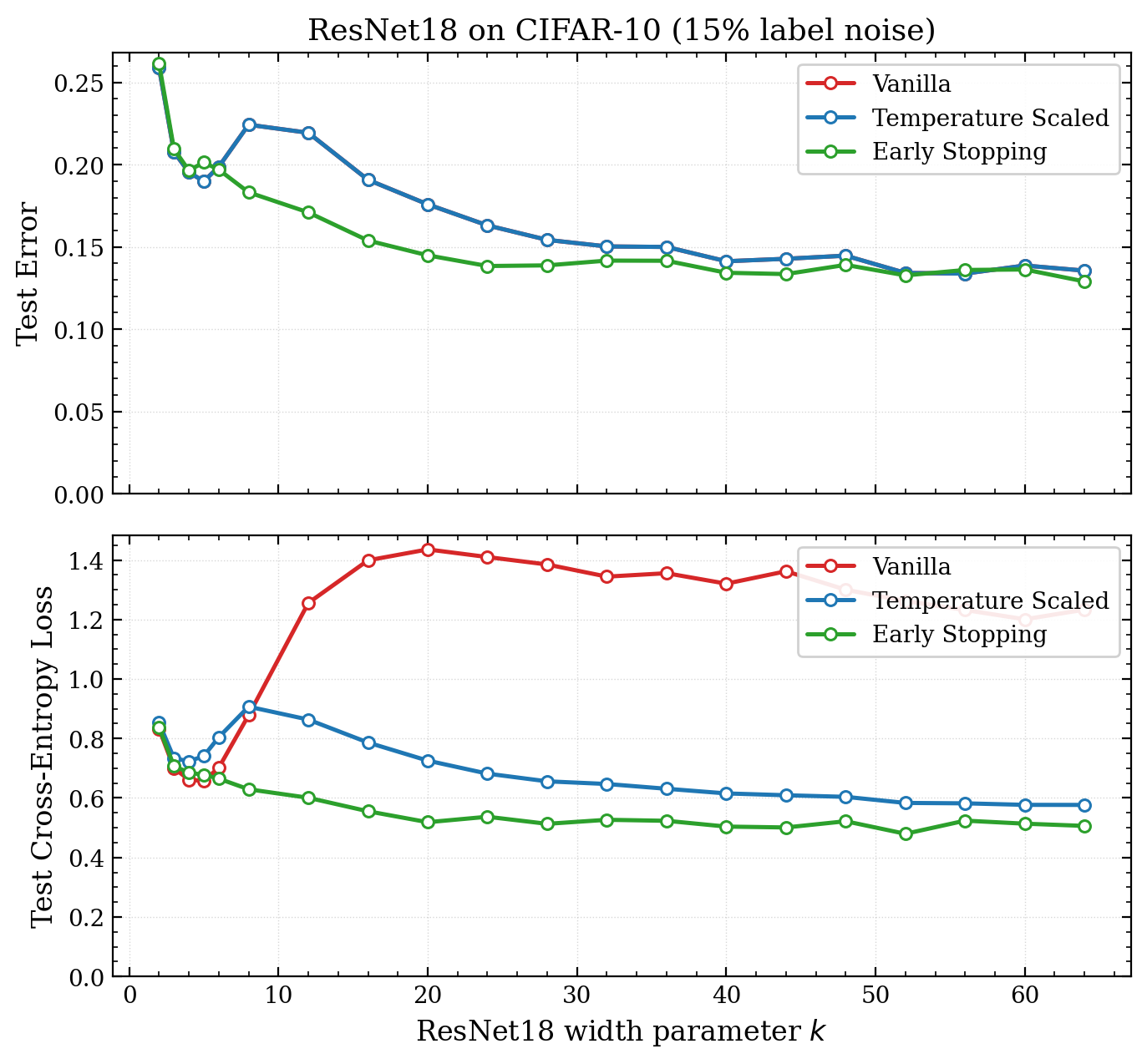
Figure 2 - The second descent regime is poorly calibrated. We replicate6 the results in Deep Double Descent [Nakkiran et. al, 2019], also showing and log loss7. It is important to note the model is trained on the 85% mislabelled CIFAR10 training set, but the test set is clean. The log loss also exhibits double descent, but the loss is much higher than the classical minimum.
Classification error (whether top1 or top5) was the eval that mattered for competitions. However it doesn’t take into account over-confidence and calibration, things that really matter in the real world. A model is well calibrated if the probabilities it produces accurately reflect the probability it is correct.
The log loss reflects how well calibrated the model is8. In addition, the log loss better captures how well the model captures the distribution (important as a base for post-training). Thankfully, both early stopping and temperature scaling Guo et. al, 2017 resolve this.
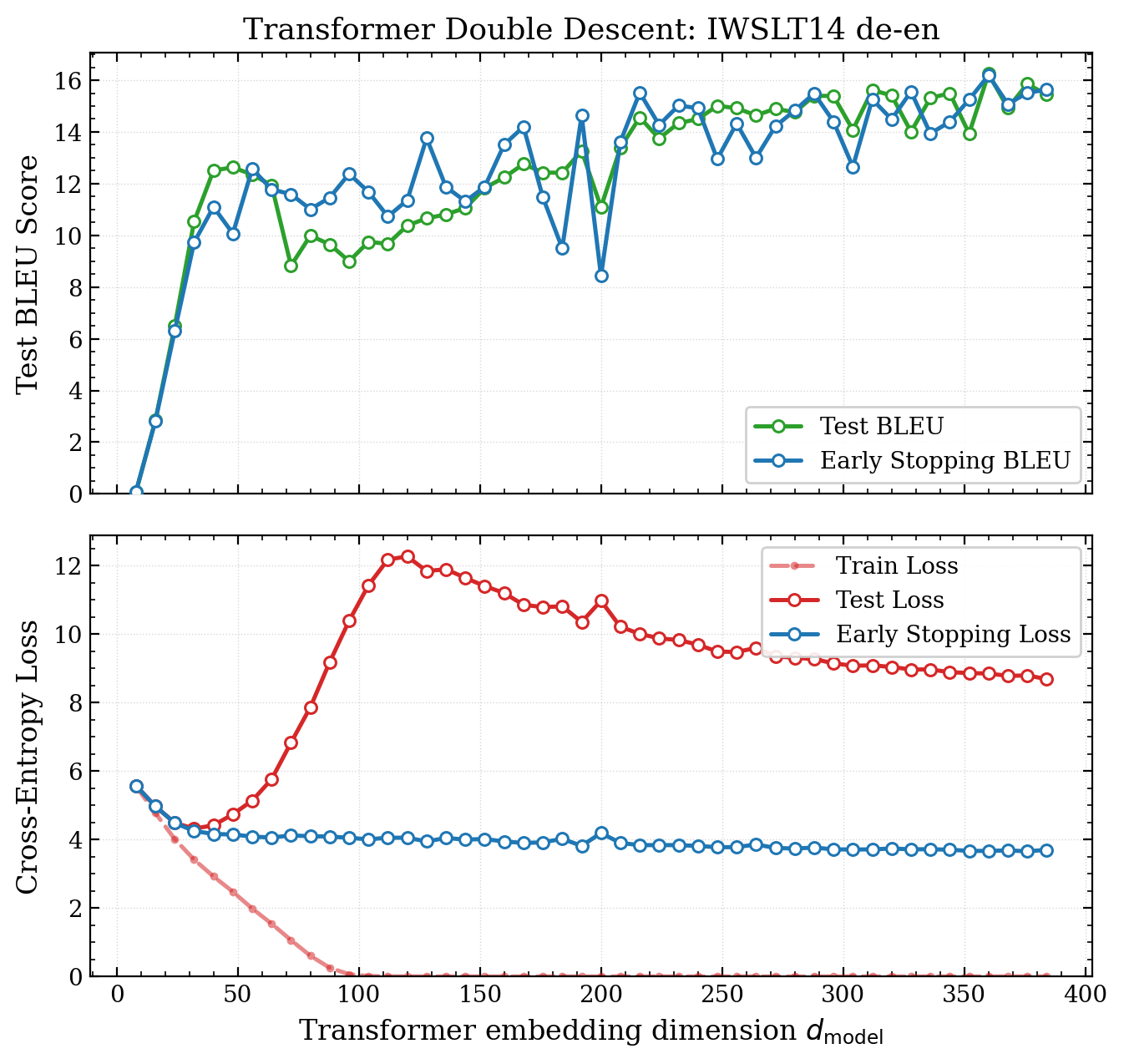
Figure 3 - Early stopping eliminates double descent for both the loss and accuracy - I retrain the Resnet18 models on 45K/5K train/val split (so we can get a validation set). The slightly smaller training set does not change accuracy much. Then we calibrate the model with temperature scaling on the validation set9. Early Stopping completely eliminates the double descent effect.
All of that was to say that early stopping makes both the error and the loss monotonically decreasing in the model size.10 Early stopping is trivial to implement, so a researcher can simply turn up the compute dial (increasing model size) and get better results.
Transformers
The deep double descent paper also demonstrates the phenomenon in the original sequence to sequence transformer architecture Vaswani et. al, 2017. I execute a similar training run to them but double the amount of sequence pairs used (18K -> 36K) so we can get a clear view of the classical regime:
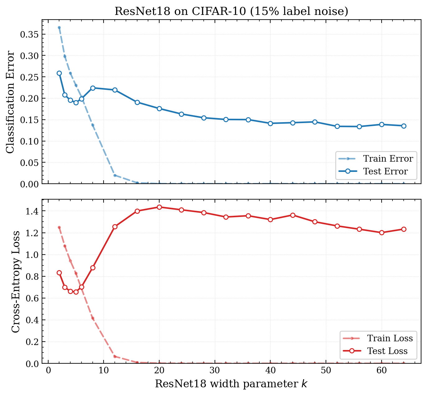
Figure 4: Transformers also exhibit monotonically increasing performance with respect to model size - Double descent is observed, trained on 36K sequence pairs from ISWLT14 english-german. The architecture used closely mirrors the original transformer architecture, following the approach in the double descent paper. However, we train with the more modern AdamW, and remove label smoothing which distorts the logits (and turns out not to be necessary).
Once again, in terms of our evaluation metric11 and the loss, overparameterization is effective. It’s important to stress how valuable this is. Crank up the number of parameters, as long as we have early stopping in place, we get better results. This gives us more confidence to do YOLO runs, we don’t need to carefully balance bias and variance.
Back to Bias and Variance
This section gets a bit technical, if you don’t have time to get into the maths, just know that we can split the log loss into two terms, a bias like term and a variance like term, the second being an excellent metric for telling us whether a model is overfitting.
Bias and variance are defined by precise second order quantities,12 but typically used in a more general sense. Bias is the systematic error in our model. It measures the error in our expected model, over all possible training sets. Variance is the random error in our model. It reflects how much a model trained by a particular training set is expected to deviate from the expected model.
Getting precise, we want to model an unknown probability distribution , where y is the image class / the next token, and x is the image / all preceding tokens. We don’t know , but we want to estimate it using our model , where represents the learned parameters. Our estimate is produced by training on a set of n samples, .
For a model produced by a single training set, across the distribution of X we have the cross entropy loss of our estimator (where C is the number of classes):
It is important to understand D itself (the training set) is also a random variable. We only see a single training set, but we are still beholden to the variance induced by it. We must analyze our training process irrespective of the particular training set we happened to sample, i.e. the risk over all possible training sets:
We want to decompose this into 3 parts:
-
The unexplainable variation in y (entropy)
-
The systematic error in our estimate (our bias-like term)
-
The random error in our estimate (our variance-like term)
By adding and subtracting at each point x, we can separate the first term:
The first term is the entropy in y (given x), this is our unexplainable variation. The second term is the KL divergence between our target distribution and the estimate. To obtain terms for bias and variance, we need a reference to our expected model over all training sets. We can center , by adding then subtracting :
The term on the left gives us our bias-like metric, notice it does not depend on a particular training set13. It is the KL divergence between our target distribution, and our expected estimator. The term on the right is our variance-like metric. It reflects the divergence of a given training run, from the expected training run. The fact that we normalize by means it is not a KL divergence, but normalizing by is exactly what we want14, because we are interested in that divergence in the places the data actually occurs.
Coming back to the risk, we have the the final decomposition:\
Our three terms:
-
- Irreducible variation in y - The entropy of
-
- systematic error in - KL divergence of and the expected model, across all x ~ X, our bias metric.
-
- random error in - The Jensen Gap of , across all training sets , across x ~ X, our variance metric.
Getting Empirical Again
Let’s apply our decomposition to the Resnet18 and transformer on their respective datasets. To measure these quantities empirically, we’ll need to train the model on multiple disjoint training sets.
In Figure 5 we trained the Resnet18 on the full 50K CIFAR10 training set. We’ll randomly break this up into 4 training sets each of size 12.5K. For the transformer (figure 6), we trained on 18K samples from the IWSLT’14 DE-EN training set, which has about 160K examples, enough data to have 8 disjoint training sets.
We can estimate with the sample mean (where M is the number of models trained on disjoint training sets):
Much like the empirical cross entropy loss we can use the sampled y values to compute the empirical Jensen Gap (variance):
For the sake of readability, I have omitted the indices inside the sum. Each x is the ith input in the mth model’s training set. y has those indices too, and a class index. y is 1 for the true class / token and zero elsewhere.
Of course, we do not know or for that matter. We cannot compute our bias term separately from the entropy. has nothing to do with our model, it is intrinsic to the data, so we know that it remains constant as we vary the number of parameters. So by observing loss - variance = entropy + bias as we increase model size, we can deduce the change in the bias:
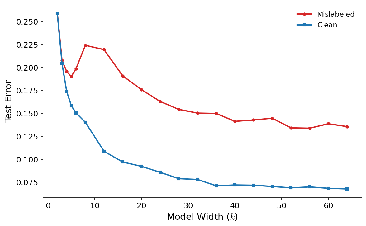
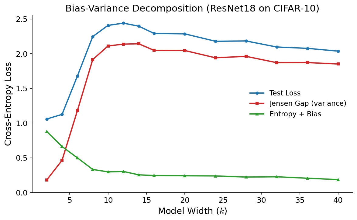
Figure 5: Resnet18 model variance dominates as model size increases - We plot the mean test loss, Jensen gap and their difference computed across 4 models, trained on 4 disjoint training sets at increasing model widths. Aside from the training set size, the setup is exactly the same as in figure 2. For low k, we observe the classical bias variance trade off (given the low sample size we miss the classical minimum in the loss). As k increases into the double descent regime, we see that bias and variance both decrease.
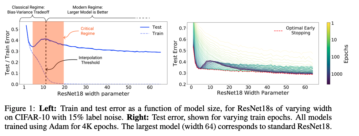
Figure 6: Transformer bias and variance both rise and fall with double descent The same 3 quantities are plotted, this time with 8 different models trained on 8 disjoint datasets of 18K sequences. Interestingly, bias also rises as we approach the loss peak.
Interpretation
If there’s anything to glean from figures 5 and 6, it’s that we shouldn’t believe simple stories about bias and variance. Yet there is a good reason for the difference. Remember there are three interesting things about our modified CIFAR10 dataset:
-
Without mislabelling, there is no double descent in test error.
-
15% of the training set is mislabeled
-
That mislabeling is not applied to the test set (it’s clean).
This means the double descent bump must be induced by the mislabelled points. The test set is clean, so any failed classification is genuine degradation. Figure 7 shows the difference between a clean trained model and our dirty one:
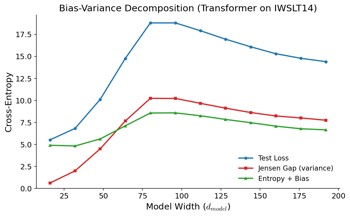
Figure 7: The effect of adding mislabelled data We show two models here both trained on the exact same set of clean examples. The red line shows our original Resnet18, the blue only subtracts all the mislabelled examples. Both are evaluated on the clean test set.
The general downward trend matches the bias, furthermore mislabelled points are completely random, so there is no way they would show up anywhere but the model variance. Each model is learning its own spurious relationship to the false labels.
Mislabeled CIFAR10 makes for a great experiment because it effectively separates explainable and unexplainable variation, making training examples either 100% explainable by a Resnet or 10% explainable (random).
With the transformer in ISWLT14 double descent showed up naturally. Token prediction15 does not have such certainties. Unlike CIFAR10 classes, most tokens do not have a probability near 1, the true16 distribution is nearly always smooth across multiple tokens. It also follows that explainable and unexplainable uncertainty are nearly always part of each token prediction.
As we head past the classical minimum, the transformer is spuriously fitting unexplainable noise causing the increase in variance. Unlike with CIFAR10, the bias is increasing too. This means the models must be identifying some structure (explainable variation) but attributing that to the wrong features.
Why does the double descent bump drop down again? That is the subject of an entire post itself, and is still somewhat an open question in the literature. The best hypothesis I have is along the lines of Wilson & Izmailov, 2020, the overfitting can be seen as a posterior over many noisy distributions, which cancel each other out with enough model capacity. The double descent bump is just the awkward point where that noise dominates.
LLM Pretraining
Imagenet, with a million images, seemed like an absurd amount of data at the time. Yet relative to compute, it really wasn’t. Researchers eventually found scalable architectures applying techniques like batch norm and skip connections. Through larger models, the compute was scaled, but the dataset remained fixed. The Imagenet-winning Resnet152 He et. al, 2015 had 60 million parameters, a 60:1 ratio of parameters to training examples.
The parameter to data ratio that LLMs and even the original transformer were trained with are fundamentally different. In our training run in figure 5 at ~30 output tokens per sentence, 36K sentences, we’re training on about 1M output tokens17. Our classical minimum was at d=32, with 515K parameters, a 1:2 p to n ratio. Double descent did not start until d=152 (6 million parameters), a 6:1 p:n ratio.
The largest model from the original transformer paper Vaswani et. al, 2017 trained on 36M sentences, approximately 1B output tokens, with only 213M parameters. That ratio is 1:5, even lower than the classical minimum for our scaled down version of that architecture. Furthermore the model is only trained for 7 or so epochs (we train ours for about 150). So despite being capable of overparameterization, it was not used to train the original transformer.
Pretrained LLMs take this further still, first of all each output token is only visited once, i.e. training is a single epoch. As prescribed by the Chinchilla scaling laws Hoffman, Borgeaud, Mensch et. al 2022, the optimal parameter to token ratio is 1:20. While that was computed for a particular dense, large scale open weight MoE’s tend to have a ratio around that number18.
Even if you tried to argue that the 1:20 parameter was still high, it is simply not feasible to drastically overfit the training loss when you visit each output token once.19 Compared to the flagship Resnet, that’s a 3 order magnitude change in the ratio.Pre-trained LLM’s are well and truly, well-parameterized, and well-calibrated OpenAI, 2023.
LLMs are Low Variance
We can use the same bias-variance decomposition on a pretrained-LLM. We fork Kaprathy’s nanochat to obtain some cheap to train LLMs. For d_model = 8, 10, 12 we train 8 models on 8 disjoint datasets from ClimbMix20, each at their compute optimal number of tokens21. Table 1 shows the loss, bias and variance:
| Depth | Min Loss | Max Loss | Mean Loss | Bias | Variance | Variance % |
|---|---|---|---|---|---|---|
| 8 | 0.9434 | 0.9453 | 0.9444 | 0.9066 | 0.0378 | 4.00 |
| 10 | 0.8923 | 0.8943 | 0.8932 | 0.8582 | 0.0350 | 3.91 |
| 12 | 0.8460 | 0.8484 | 0.8473 | 0.8150 | 0.0323 | 3.81 |
Table 1: Bias variance decomposition of pre-trained LLMs22 - We see that at the compute optimal point, the loss is dominated by the bias. Variance makes up a small fraction of the loss.
Table one conclusively shows pre-trained LLMs are well-parameterized. The low variance is a testament to the power of pre-training, take two different datasets drawn from the same pre-training corpus, and you’ll more or less get the same model. This also explains why despite being trained by different organizations, pre-trained models are remarkably similar.
From the Data Bottleneck, to the Compute Bottleneck
When AlexNet first made deep learning work at scale, it took a few years of algorithmic improvements to get the most out of the data. All the models from Alexnet (2012) to Resnet152 (2015) used the same fixed training set, trained for about 100 epochs. Notably, Alexnet and Resnet152 both have about 60M parameters. There was so much compute latent within the GPU, we just needed the right algorithms to use it.
As the algorithms got better, we eventually saturated Imagenet. At that point our data is what limited us. OpenAI correctly internalized this, and bet the house on unfiltered internet data. A trillion token data source that also happens to contain most of humanity’s knowledge. Data is no longer the bottleneck, nor is that the case in post-training (talking about quantity here, not the type of data)23.
In the mid 2020’s, it is still the case that increasing compute and data in lockstep yields a better log loss (and downstream results). We are yet to see saturation there.24 Even if we “ran out of data” to get more from pre-training we could crank up the epochs once again. Our real constraint today is compute. Large models cost more, take longer to train, post-train and iterate over. The scale of the models is starting to move in lockstep with compute, with models from the frontier labs reportedly now only exceeding the original GPT4 size.
Whenever data is constrained, or compute is constrained, we rely on better algorithms, or different kinds of data to make progress. In the era where progress was driven by CNN’s we had ample compute but fixed (and with hindsight small) datasets. Switching to next token internet data removed the data bottleneck, but after scaling for some years we’ve hit the compute bottleneck.
When to Overfit?
Let’s summarize:
-
For transformers and CNN’s, we’ve seen that models continue to perform better and be better calibrated as parameter count increases.
-
However in data rich environments like LLM pre-training, we are better off adding more data, rather than overparameterizing, because it is a more compute efficient way of obtaining better performance.
So for deep learning25 overparameterization is broadly effective, provided you are willing to pay the computer for it. A prominent example of a data constrained domain today is medical image segmentation, where for a variety of reasons, it is difficult to obtain datasets. Convolutional U-Nets Ronnenberger et. al, 2015 are still the state of the art for image segmentation (see Ulrich et. al, 2024).
In the original U-Net paper, there are 30 million parameters for a training set of 30 images, a million to 1 p:n ratio! U-Nets do train pixel by pixel,26 even per pixel the ratio is still 4:127. There is no large dataset or base model to leverage in this domain. The very limited access to data means it makes sense to crank up the parameter count and utilize that GPU.
Overparameterization will continue to help the niche economically valuable modalities28 which lack data. What about general frontier models? In the realm of post-training, I suspect overparameterization and questions of sample efficiency will be important.
We currently favour the dataset types that scale, doubling down on pre-training, emphasizing RLVR over RLHF. On the road to AGI, there is likely some types of data we need that do not scale. Here, we may stand to benefit from deep learning’s ability to explore a complex model space with low variance. At any rate, overparameterization in post-training requires separate treatment, and will have to wait for a future post.
Footnotes
-
We use overparameterization in the simple sense of a high number of parameters p, relative to the number of training examples / target tokens n. ↩
-
With a fixed dataset ↩
-
See Hastie et. al, 2022 and Bartlett et. al 2020 ↩
-
See section 10.4. 2 on page 34 of McKay, 1995 ↩
-
a.k.a aleoteric uncertainty ↩
-
I modified the training recipe slightly to make use of modern optimizers (AdamW) to converge faster, see the code for more details. Nonetheless, the results are the same. ↩
-
Nakkiran et. al did show test loss in their appendix, the result is the same as our graph here. ↩
-
A useful metric to look at when studying calibration in classification is Expected Calibration Error (ECE) Guo et. al, 2017, which splits the data into bins based on confidence, and asks how closely the correctness percentage in the bin matches the confidence output by the model. Recall training set (and validation set) is perturbed with a 15% random mislabelling, while the test set is clean. This means the test distribution is in fact different. This renders ECE on the dirty validation set underconfident, so it is not a useful metric for our particular setup. Nonetheless, as discussed in Guo et. al, 2017 the log loss is an effective score for calibration. Furthermore once we get to token prediction, ECE is not usable because the vocab size relative to the validation set renders most per class bins empty. ↩
-
Recall that temperature scaling is a constant scale applied to the logits, as such it never changes the prediction and cannot change the accuracy. ↩
-
More strictly its width, for this architecture ↩
-
BLEU score, a measure of translation quality. ↩
-
Bias and Variance are more precisely described in the context of the Mean Squared Error, as it can be decomposed exactly into those quantities: Bias =(p(x)-E_Dq(x))^2 , Var = E_D(E_Dq(x)-q(x))^2 ↩
-
In the denominator we have integrated over all possible training sets. ↩
-
and a mathematical necessity ↩
-
Whether next token or sequence to sequence ↩
-
“True” is of course a bit of a misnomer as Bayesians. ↩
-
Output tokens are the relevant n here because they dictate the number of training examples. That is, each token in the output sentence corresponds to a training example. ↩
-
That is total parameters (not active parameters). Total parameters is the relevant parameter count for model expressiveness. ↩
-
and the training losses for large LLM training runs show this, they’re just not that different from the validation loss. ↩
-
See Nvidia, 2025 ↩
-
This is a departure from the fixed dataset analysis we have done so far, but we want to see the model variance at the point LLMs are actually pretrained at, which is nearly always around the compute optimal p:n ratio (varies per model). ↩
-
I apologize for showing only 3 points but I am compute poor ↩
-
I do believe we are bottlenecked on the kind of data we have. For example there was a lot of useful feedback in the human evolution process that is difficult to replicate in the case of models. ↩
-
That said, the log loss cannot go down forever, the limit is the unexplainable entropy in the next token (given the preceding tokens) - H(Y | X). ↩
-
Prescribing this to deep learning writ large is an overstatement, we’ve not shown this for every architecture. ↩
-
or voxel by voxel ↩
-
Yes each Pixel is labelled but medical image segmentation datasets are severely class imbalanced. The vast majority of pixels are 0 labels (normal human tissue), so to call the ratio 4:1 would be overcounting data points. ↩
-
At least until more general models are able to operate across all these modalities effectively. ↩